Warehouse storing route optimization with Reinforcement Learning
 Optimization of the robots route for pick-up and storage of items in a warehouse
The problem represents a storage decision process where outcome is under the control of a robot, i.e, a decision maker agent, but also are partly random. Therefore, the problem can be well modeled as a discrete-time Markov Decision Processes. The approach follow was:
- Implement a reinforcement-learning based algorithm
- The robot is the agent and decides where to place the next part
- Use the markov decision process toolbox for your solution
- Choose the best performing MDP
Defitinions
The basic concepts to understand the promblem are shortly introduced based on Artificial Intelligence: A Modern Approach book:
-
Reinforcement learning: Type of dynamic programming that trains algorithms using a system of reward and punishment. The agent learns without intervention from a human by maximizing its reward and minimizing its penalty and updates itself continuously. The algorithm it automatically finds patterns and relationships inside of that dataset. It requires realtime data.
-
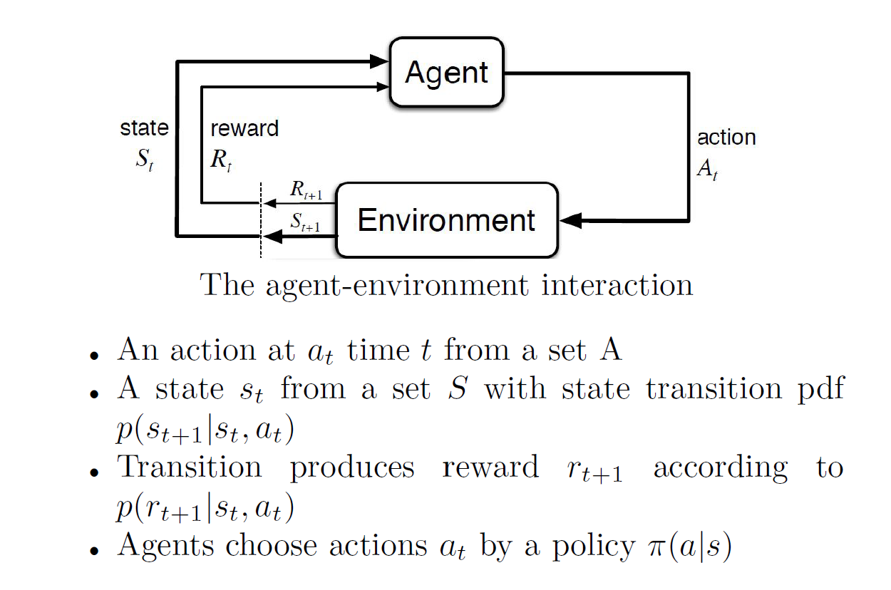
Agent: A is the set of all possible moves the agent can make. An action is almost self-explanatory, but it should be noted that agents choose among a list of possible actions.
-
Environment: The world through which the agent moves. The environment takes the agent’s current state and action as input, and returns as output the agent’s reward and its next state.
-
State: The parameter values that describe the current cofiguration of the environment, which the agent uses to choose an action. A state is a concrete and immediate situation in which the agent finds itself; i.e. a specific place and moment.
-
Reward: Feedback by which we effectively evaluate the agent’s action. From any given state, an agent sends output in the form of actions to the environment, and the environment returns the agent’s new state (which resulted from actingon the previous state) as well as rewards, if any. Rewards can be immediate or delayed.
-
Markov decision process: Markov decision processes (MDPS) is a model decision making in stochastic, sequential environments. The essence of the model is that a decision maker, or agent, inhabits an environment, which changes state randomly in response to action choices made by the agent.
Example Introduction
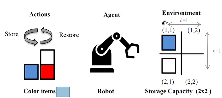
A tiny warehouse with (2x2) storage capacity locations is simulated. The picking robot (agent) interacts with the warehouse (environment) by store-restoring items in each warehouse cell or shelve. The dataset contains store and restore action for red, blue and white colored items although an empty field is also possible.
When the agent is placed on a field position (𝑥𝑑, 𝑦𝑑), it can either store or restore each of the color items. There exists a total of six possible actions to change its environment. The robot can move in the (2x2) grid environment and start moving at initial grid position (1,1) . The robot is constrained to always to move only to one adjacent fields (not in diagonal).
The distance the robot needs to move is derived based on current (𝑥𝑐 , 𝑦𝑐 ) and goal position (𝑥𝑑 , 𝑦𝑑). The distance is calculated as the sum of the absolute differences of the layout position $$ 𝑑 = |𝑥_𝑑 − 𝑥_𝑐 | + |𝑦_𝑑 − 𝑦_𝑑|$$
Therefore, the distance to the position can be assigned to the cost of the action or negative reward. The ideal goal of the reinforcement learning approach would be to optimize the route picking storage strategy by minimizing the distance with rewards the store/restore motion actions.
Methods
The Markov Discrete Process (MDP) algorithm was implemented for modelling the problem. A MDP is described by state transition probabilities. A general Reinforcement Learning and thus also MDP algorithm is defined with a set of variables:
-
Actions (A): refers to the operations an agent can perform which direct modify the environment. In our problem this are related to the effect on the warehouse grid cells, directly proportional to the warehouse size (𝑋, 𝑌). $ A = \{ 𝐴_{(1,1)}, 𝐴_{(1,2)}, 𝐴_{(2,1)}, … , 𝐴_{(X,Y)}\}$ where $ |𝐴| = |𝑋 \cdot 𝑌|$ .
-
States (S): represent all the possible configuration of environment, i.e, how the items are storage in the warehouse grid. In the addressed problem, the total states can be computed $ |S| = \{𝑖𝑡𝑒𝑚𝑠_{𝑔𝑟𝑖𝑑}*move_{action} \}$ where the items on the grid is calculated as the exponential relation of colored items number to grid size, and the move actions represent all the possible robot movements {store: blue/red/white, restore: blue/red/white }.
-
Transition probability matrix (TMP) in Markov processes stores the probability to transition from the current state to a next possible state after the agent has performed given action in a single time unit. The dimension if this matrix is determined by (|𝐴|,|𝑆|,|𝑆|).
-
Reward matrix (R), is composed by the defined reward or symbolic benefit received performing and action 𝐴(𝑥,𝑦) for a given state. The shape of this matrix (|𝑆|,|𝐴|).
Transition Probability Matrix (TPM)
In the simple addressed problem, the warehouse grid is of size the 2x2. Therefore, so have 2·2=4 possible actions and 1536 different states. In order to compute the probability actions, is necessary to iterate through all possible actions as well as all generated states. Then assign the possibility of having a colored item or being empty derived from the training data frequencies. It should also be taken into account if the warehouse grid is already full and if the linked operation is invalid. In that case, the transition probabilities are kept 0. To assert that the computation was correct, it was checked that all he probabilities for a particular state sum 1.
Regard Matrix
The aim of the reinforcement learning algorithm is to maximize the obtained rewards. In this problem, the distance should influence the reward. Thus, the simple criteria to assign the negative distances values from the origin warehouse cell (1,1). At the same time, not from every state the robot can transition to other state. For the entries in the reward matrix, as the movement action would be invalid, a penalization of -10000 was taken as a reward. With the necessary TMP and R, a MDP model is trained within the python-MDPtoolbox package. It contains the most common Reinforcement Learning training approaches, such as Value Iteration and Policy Iteration. These were the best models selected for the simplified problem. The discount factor and maximum iteration hyperparameters were set to 0.9 and 750 respectively.
Evaluation
MDP policy refers to a solution to which specifies an action for each state. Value iteration is defined as an algorithm that gives an optimal policy for a MDP, i.e., The ideal MDP solution. In the training run, for policy iteration 6 iterations were performed whereas for value iteration 35 were performed. To evaluate the model, a test dataset containing 60 pair of movement actions and colored items was used. Although different MDP algorithms were tried, there was no change on the result. The movements distance need was 232 for both Value Iteration and Policy Iteration. That may be due to on the restricted problem, the simple algorithm is already learning the optimal policy for the given rewards. In order to assess if the policy represents a better utility than random, a simple random walk approach through the grid was also implemented. In that the distance or movements performed by the robot are count. The random distance, although the random seed was fix, it rounds the range of 264.
| Algorithm | Move Distance |
|---|---|
| Value Iteration | 232 |
| Policy Iteration | 232 |
| Random Walk | 264 |
Maria Monzon
Computer Vision and AI researcher
My research interests include Computer Vision, Biomedical Image Analysis, Trustworhty Deep Learning and Machine Learning for healthcare.