Financial Transaction Text Clasifier
 Multinomial Bayes Text Clasifier
The aim of the project is to classify financial transactions, stored in a datasheet file, into one of seven categories listed:
- Income
- Private (cash, deposit, donation, presents)
- Living (rent, additional flat expenses, …)
- Standard of living (food, health, children, …)
- Finance (credit, bank costs, insurances, savings)
- Traffic (public transport, gas stations, bike, car …)
- Leisure (hobby, sport, vacation, shopping, …)
The selected approach is to train a Multinomial Naive Bayes classifier, fitted with the transaction word counts and class categories. Naive Bayes is a statistical classification technique based on Bayes probability theorem, considered as one most basic supervised learning algorithm. Naive Bayes classifier assumes that the features in a class are independent of other features. The followed approach to implement the classifier can be is based on the standard steps of Machine Learning (ML) algorithms: data exploration and preprocessing, feature selection and transformation, classifier model definition and training. The final phase of the assignment is dedicated for results visualization and evaluation.
Data exploration and preprocessing
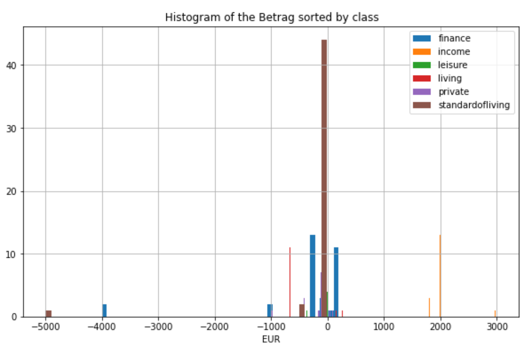
The essential first step is to import the dataset files into the python program, loaded as a pandas DataFrame data structure. The next step performed was a data quality assessment by printing the header columns, missing values datatypes and a short overview of the data samples. Furthermore, the unique values of each field as well as the label frequencies are printed to determine if the dataset suffers from class imbalance. As a quality assessment result, data cleaning procedures were performed. The missing values were substituted the missing values with 0, to minimize the effect of these on the accuracy of the model. For the text fields, the data was standardized by removing capital, special and/or punctuation characters, German stopwords and 2 or a single character-words. Finally, the sentences were splitted into single words (tokenize). After the data cleaning and preprocessing, to check if the process was done successfully, a final data inspection and a summary of the dataset by class was depicted. A secondary reason for the data inspection was to have an insight of the feature’s distributions and outlier identification.
Feature transformation
Feature transformation refers to translating the data into an appropriate format allowing the ML model to learn from the data. For instance, categorical data need to be converted to numerical data for the Naïve Bayes classifier. The categorical labels were converted to values ranged between 0-5. A common step in ML is also feature selection, i.e selection of the features in dataset hypothesized to be the most descriptive. Therefore, all the numeric values were scaled between the range 0-1 to reduce the variance. The string features were vectorized and concatenated to create the feature matrix. The final feature dimension was 502. As an optional step, a model selector of the best K features was also implemented for feature dimensionality reduction.
Model Training
The selected classifier model is a Multinomial Naïve bayes classifier implemented in the sklearn library. As only few data samples were available in the dataset, a cross validation scheme has been used for training and evaluation. The data was splitted in k=10 folds and with stratified sampling to mitigate the class imbalance. Note that even the predict phase was done in after fitting the classifier on the KFold iteration, but this does not interfere in the training process.
Evaluation and Result visualization
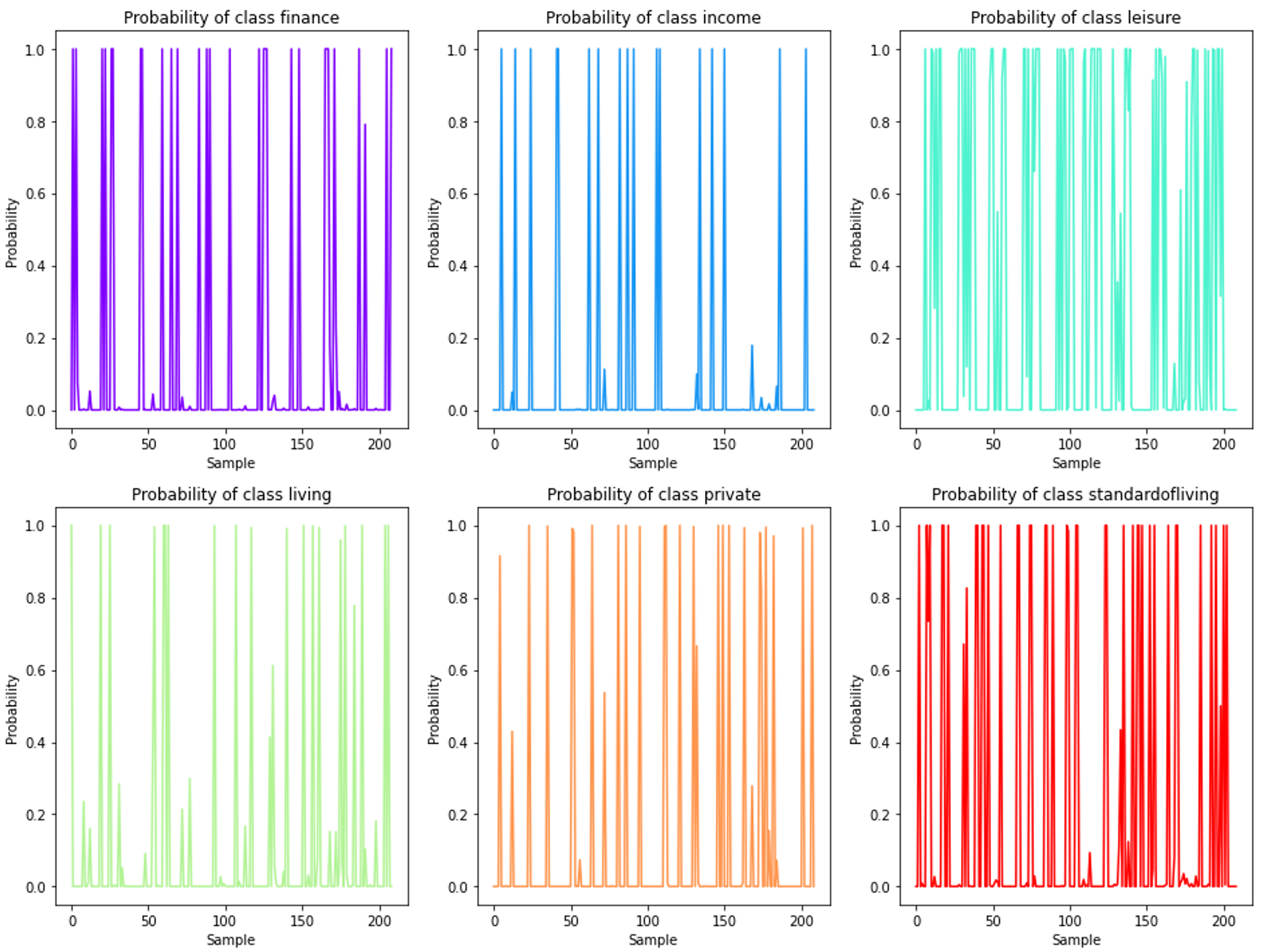
As stated previously, the data samples present in the datasheet are not many to test the robustness of the classifier a cross validation scheme has been used for evaluation. For each class, the predicted probabilities are plotted in the next figure. The probabilities for each sample are close to 1, which resembles the a extreme probability assignament of Naïve Bayes Classifier.
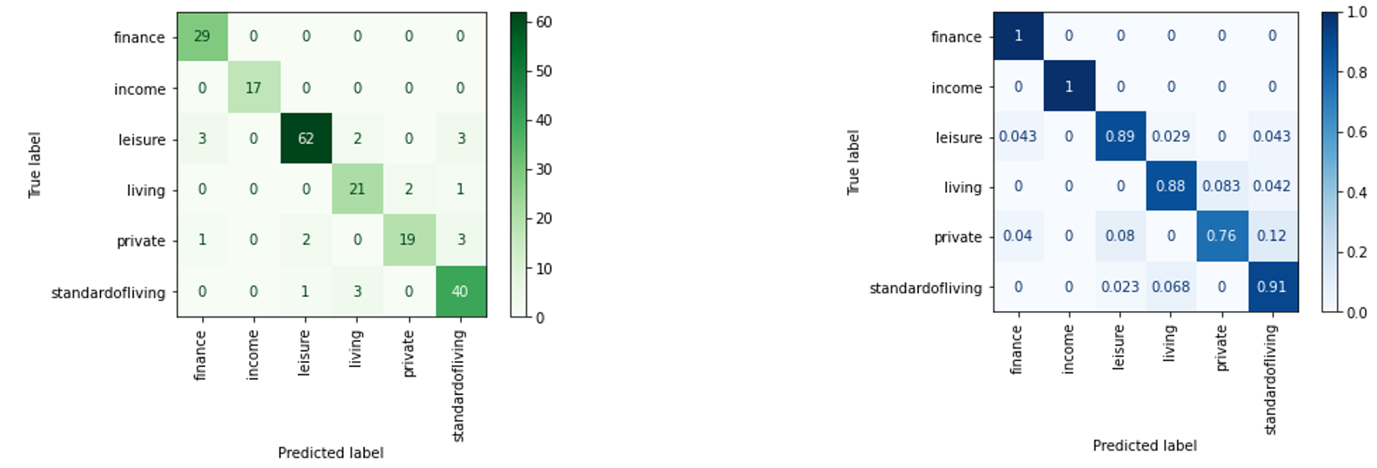
In order to quantified the performance of the classifier, many quantitative metrics were computed. The most common evaluation method in classification is the so-called confusion matrix. The Matrix is represented for a binary classification although it can be extended to multiclass problem. The matrix represents the relation between correctly classified, i.e. true positives (TP) and True Negatives (TN), and wrongly predicted samples , i.e. false negatives (FN) and false positives (FP) for each class. The matrix can be displayed with absolute frequency values or normalized by each class total number of elements. The confusion matrix for the assignment are shown below:
From the confusion matrix to assess the the quality of the predictions further evaluation metrics can be derived, a ranged from 0 to 1 (represents the best possible score):
-
Accuracy: metric of all the correctly classified samples over the total number of samples that asses the overall performance of the model $$ Accuracy = \frac{TP+TN}{TTP+TN+FP+FN}$$
-
Precision: proportion of correctly predicted samples (TP) to the total predicted samples as positive, therefore assess the correct prediction capability for each class. $$Precision= \frac{TP}{TP+FP}$$
-
Recall: ratio of correctly predicted samples (TP) and actual total samples of such class, therefore an assessment metric of the ability to classify all correct instances per class. $$ Recall = \frac{TP}{TP+FN}$$
-
F1-score: is the harmonic mean between precision (P) and recall (R) and asses the incorrectly predicted samples, especially in class imbalanced problems $$Precision= \frac{2 \cdot P \cdot R}{P+R}$$
The model achieves a total weighted accuracy of 90% and an averaged F1-score of 90%. The detailed evaluation metrics for each class are summarize in the following table:
| Label | Total Samples | Precision | Recall | F1-score | |
|---|---|---|---|---|---|
| Finance | 33 | 1.00 | 0.88 | 0.94 | |
| Income | 17 | 1.00 | 1.00 | 1.00 | |
| Leisure | 65 | 0.89 | 0.95 | 0.92 | |
| Living | 26 | 0.91 | 0.81 | 0.86 | |
| Private | 21 | 0.77 | 0.95 | 0.85 | |
| Standard of living | 47 | 0.91 | 0.85 | 0.88 |
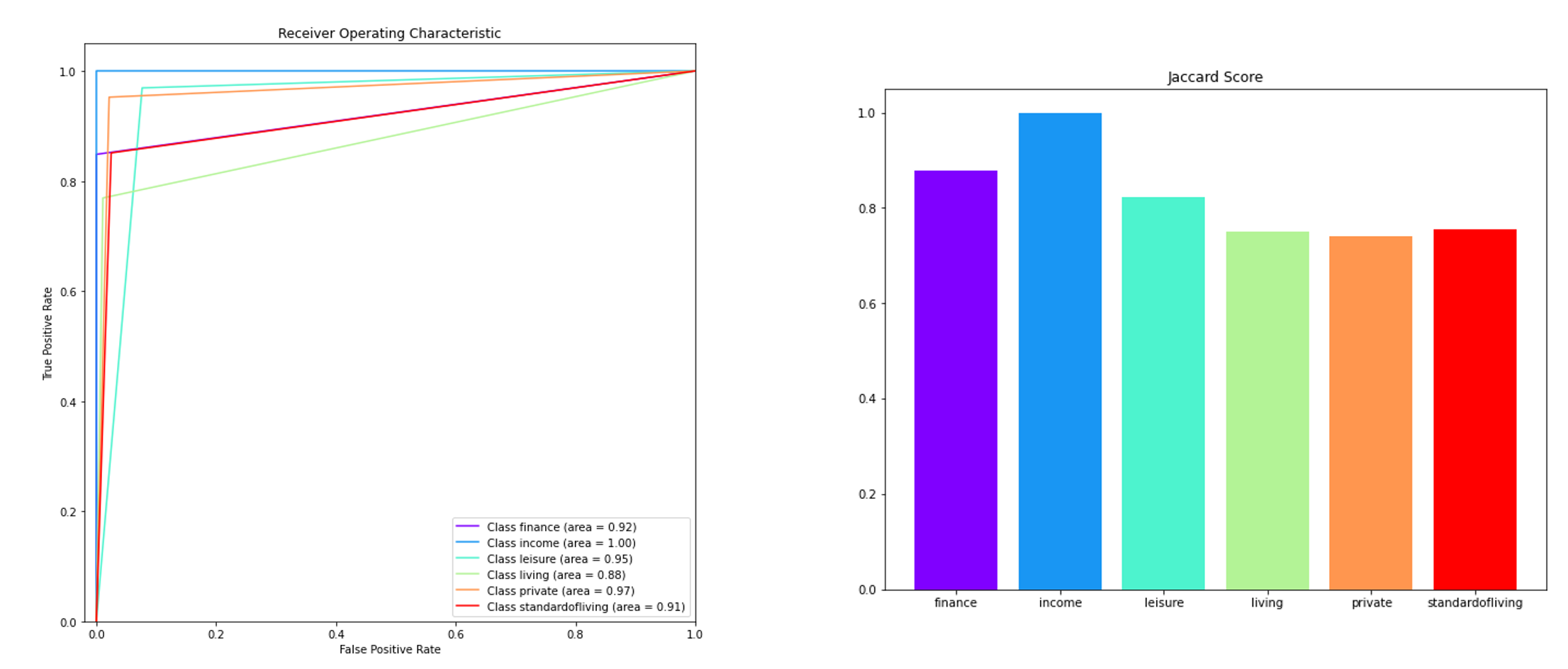
For further visualization of the results, two additional graphic representations are shown in Figure 3. A Receiver Operator Characteristic (ROC) curve is a representation to assess the performance of binary classifiers, but it can be adapted for a multiclass classification by computing a curve for each class. The curve was computed following one-vs-all approach so that each class considers that class label as a true and all others as negative. From this curve, a further metric is usually derived as a summary of ROC, the area under the curve (AUC). When AUC value is 1, it means that the classifier is able to classify all the classes, on the contrary, when the values is 0.5, the classifier only can classify a random label or a constant value. As depicted in the evaluation ROC, for all classes the AUC measures are over 0.88. Furthermore, the Jaccard similarity is a similarity metric for samples of two class sets to determine which samples are shared and which are distinct. It is defined as the number of the label intersection divided by the union of two label sets.
Maria Monzon
Computer Vision and AI researcher
My research interests include Computer Vision, Biomedical Image Analysis, Trustworhty Deep Learning and Machine Learning for healthcare.